SUMMARY: Calculating hours worked in Excel is a foundational workplace skill that empowers employees, managers, and small business owners to accurately track time, compute payroll, and analyze productivity. This guide walks you through every method — from basic time subtraction and the TEXT function to advanced techniques like handling overnight shifts, using NETWORKDAYS for business hours, building automated timesheets, and avoiding common pitfalls around Excel’s time formatting system. Whether you are creating a simple daily log or a full-featured weekly timesheet with overtime calculations, this guide covers all the formulas, functions, and formatting rules you need to get accurate results every time. |
1. Understanding How Excel Stores Time (The Foundation)
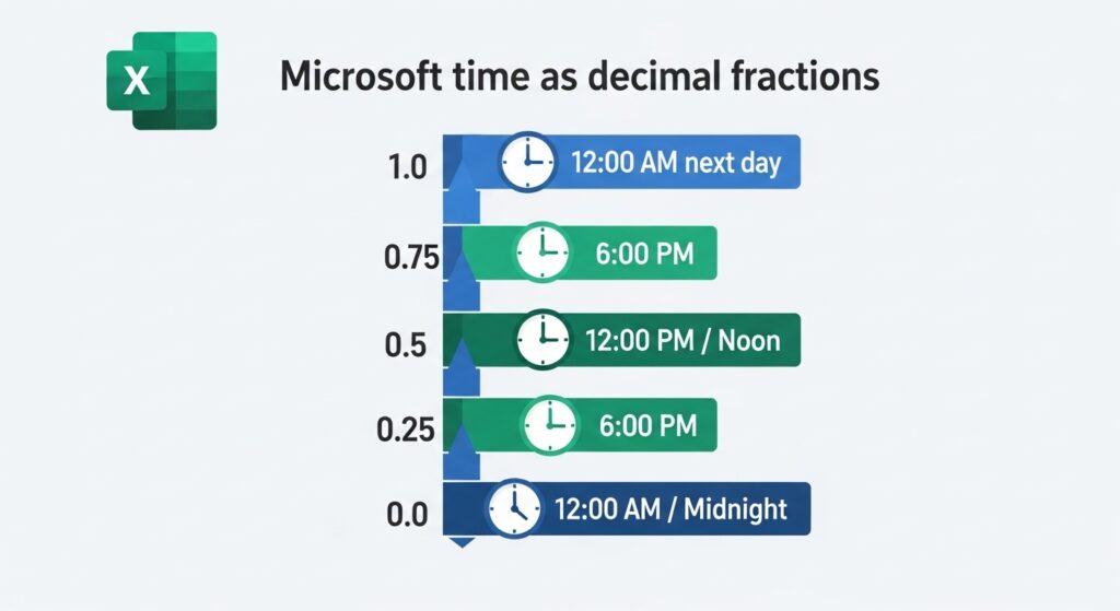
Before diving into formulas, you must understand one critical concept: Excel stores time as decimal fractions of a 24-hour day. This is the root of almost every time calculation question and formatting confusion that Excel users encounter.
How Excel’s Time System Works
In Excel’s internal system:
- 1.0 = 24 hours (one full day)
- 0.5 = 12 hours (noon)
- 0.25 = 6 hours
- 0.0417 ≈ 1 hour
So when you type “8:00 AM” into a cell, Excel stores it as 0.333333 (8 ÷ 24). When you type “5:00 PM,” it stores 0.708333 (17 ÷ 24). Subtracting these gives 0.375, which equals 9 hours.
Why This Matters for Your Calculations
If you skip this understanding and format your results incorrectly, Excel will display something like “0.375” instead of “9:00” or “9 hours.” Throughout this guide you will see how cell formatting controls whether your result looks like a fraction, a clock time, or a clean decimal number.
| 💡 Key Insight: Excel’s time values are always fractions of a day. Multiply by 24 to convert to decimal hours. Format cells as [h]: mm to display hours and minutes cleanly. |
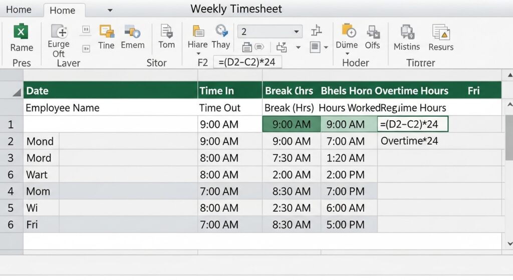
2. Setting Up Your Timesheet Spreadsheet
A well-structured timesheet is the foundation of accurate time tracking. Getting the layout right before entering formulas saves significant troubleshooting time later.
Recommended Column Layout
| Number or [h]: mm | Label | Example Data | Format |
|---|---|---|---|
| A | Date | 04/01/2025 | Date |
| B | Employee Name | John Smith | General |
| C | Time In | 9:00 AM | Time (h:mm AM/PM) |
| D | Time Out | 5:30 PM | Time (h:mm AM/PM) |
| E | Break (hrs) | 0.5 | Number |
| F | Hours Worked | [Formula] | Number or [h]:mm |
| G | Regular Hours | [Formula] | Number |
| H | Overtime Hours | [Formula] | Number |
How to Format Cells for Time Input
Step 1: Select the cells where users will enter start and end times (columns C and D).
Step 2: Right-click and choose Format Cells (or press Ctrl+1).
Step 3: Click the Number tab, select Time, and choose the format 1:30 PM or 13:30 depending on your preference for 12-hour or 24-hour format.
Step 4: Click OK. This ensures Excel interprets your entries as time values, not plain text.
3. Basic Formula to Calculate Hours Worked
The most fundamental calculation in any timesheet is: End Time minus Start Time. This is where almost every time-tracking spreadsheet begins.
Simple Subtraction Formula
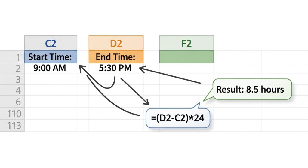
Assuming C2 = Start time (e.g., 9:00 AM) and D2 = End time (e.g., 5:30 PM), enter this formula in F2:
=D2-C2
If your cell is formatted as Time, the result will show 8:30 (8 hours and 30 minutes).
Converting the Result to Hours as a Number
To display hours as a decimal number (e.g., 8.5 instead of 8:30), multiply the result by 24:
=(D2-C2)*24
This formula converts Excel’s fractional day value into a standard decimal hour value. Format column F as a number with 2 decimal places for clean output.
Step-by-Step Example
- In A2, type the date: 04/01/2025
- In C2, type the start time: 9:00 AM
- In D2, type the end time: 5:30 PM
- In F2, enter: =(D2-C2)*24
- Format F2 as Number → Result: 8.5
4. Calculating Total Hours with the TEXT Function
The TEXT function gives you precise control over how time results are displayed, especially useful when you want to show hours and minutes in a readable format for reports and printed documents.
Using TEXT to Format Time Results
=TEXT(D2-C2,”h:mm”)
This formula displays the result as hours and minutes (e.g., 8:30). For results that might exceed 24 hours, use square brackets:
=TEXT(D2-C2,”[h]:mm”)
The [h] notation tells Excel not to reset the hour count at 24, making it essential for summing multiple days of work.
When to Use TEXT vs. Numeric Formats
- Use TEXT when the result is for display only (reports, printed timesheets)
- Use *(24) multiplication when you need to perform further math (like multiplying by an hourly rate for payroll)
- Use [h]: mm format directly on cells when you want both readability and the ability to sum values
5. Converting Time to Decimal Hours
Decimal hours are the preferred format for payroll calculations because they allow straightforward multiplication by an hourly wage rate.
The Multiplication Method
=(D2-C2)*24
| Time In | Time Out | Hours (Decimal) |
|---|---|---|
| 8:00 AM | 4:00 PM | 8.0 |
| 9:30 AM | 6:00 PM | 8.5 |
| 7:15 AM | 3:45 PM | 8.5 |
Calculating Pay from Decimal Hours
Once you have decimal hours, multiplying by the hourly wage is simple:
=F2*hourly_rate
For example, if F2 = 8.5 hours and the hourly rate is $15: =F2*15 → Result: $127.50
Converting Hours and Minutes to Decimal Using HOUR and MINUTE
=HOUR(D2-C2) + MINUTE(D2-C2)/60
This extracts the hour component and minute component separately, converting minutes to a fraction of an hour before adding them together.
6. Handling Lunch Breaks and Deductions
Most professional timesheets need to subtract unpaid break time from the total hours worked to arrive at actual billable or payable hours.
Subtracting a Fixed Break Duration
If employees take a standard 30-minute (0.5-hour) unpaid lunch break:
=(D2-C2)*24-E2
Where E2 contains the break duration in decimal hours (0.5 for 30 minutes, 1.0 for 60 minutes).
Subtracting Break Using Time Values
If you prefer to enter break times as actual clock times, with E2 = Break Start and F2 = Break End:
=(D2-C2-(F2-E2))*24
This formula subtracts the break duration from the total shift duration before converting to decimal hours.
Building a Break-Aware Timesheet (Minutes Input)
For a clean layout where a break is entered in minutes:
=(D2-C2)*24-(E2/60)
Here E2 holds break minutes (e.g., 30), divided by 60 to convert to hours, before subtracting from the total.
7. Calculating Overnight Shifts (Time Past Midnight)
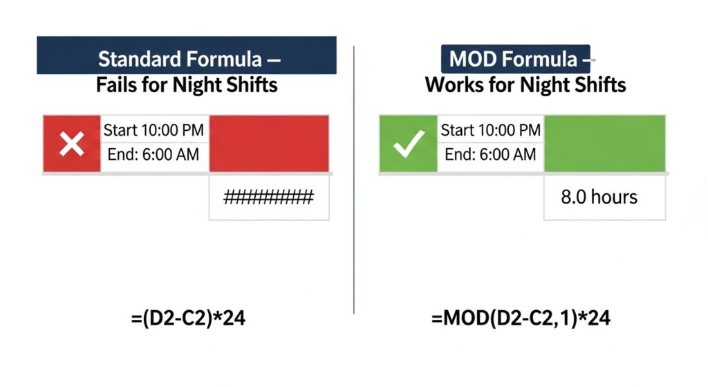
Night shift workers present a unique challenge: their end time is numerically shorter than their start time (e.g., start 10:00 PM, end 6:00 AM), which causes a negative result with simple subtraction.
Why Standard Subtraction Fails for Night Shifts
=D2-C2 → Negative result if D2 < C2
Example: 6:00 AM – 10:00 PM = -0.667, which Excel may display as ######## in narrow columns.
The IF Formula for Overnight Shifts
=IF(D2<C2, D2+1-C2, D2-C2)*24
How it works: If the end time is less than the start time (overnight), Excel adds 1 (one full day) to the end time before subtracting. If the end time is greater (same-day), it uses normal subtraction.
Using MOD for Overnight Calculation (Recommended)
=MOD(D2-C2,1)*24
The MOD function ensures the result is always positive, automatically handling both same-day and overnight shifts without an IF statement. This is the preferred, cleaner approach.
Step-by-Step Night Shift Example
- C2 = 10:00 PM (start time)
- D2 = 6:00 AM (end time, next day)
- Formula: =MOD(D2-C2,1)*24
- Result: 8 (8 hours worked overnight)
8. Summing Total Weekly Hours
Once you have daily hours calculated, summing them for a weekly total is straightforward — but formatting of the result cell is critical to getting correct results.
Using SUM for Weekly Totals (Decimal Hours)
=SUM(F2:F8)
If your hours column contains decimal values (8.5, 7.0, 9.25, etc.), this gives you total hours as a plain decimal number. Format the cell as Number.
Summing Time-Formatted Values — Critical Formatting Step
=SUM(F2:F8) → Format the result cell as [h]:mm
The square brackets in [h]: mm are essential. Without them, Excel resets the hour count at 24 hours, so 40 hours would incorrectly display as 16:00 instead of 40:00.
| 💡 Step-by-Step: Format the SUM cell correctly1. Select the total cell 2. Press Ctrl+1 (Format Cells) 3. Click the Number tab → Custom 4. Type [h]:mm in the Type field 5. Click OK |
Creating a Running Daily Total
=SUM($F$2:F2)
This uses an absolute reference for the start row and a relative reference for the end row, expanding automatically as you copy the formula down through each day.
9. Calculating Overtime Hours in Excel
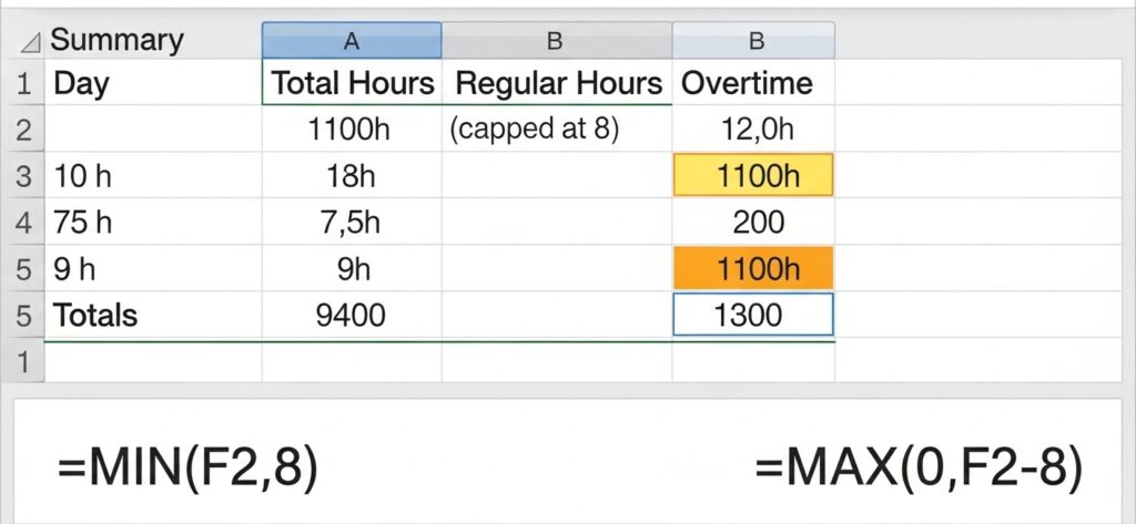
Overtime is typically defined as hours worked beyond 8 per day or 40 per week. Excel’s MAX and MIN functions handle overtime calculations cleanly and precisely.
Daily Overtime Formula
=MAX(0, F2-8)
If hours worked (F2) is 10: overtime = MAX(0, 10-8) = 2 hours. If hours worked is 7: overtime = MAX(0, 7-8) = 0 (no overtime). The MAX(0,…) prevents negative values.
Regular Hours Formula (Capped at 8 Per Day)
=MIN(F2, 8)
This ensures regular hours never exceed 8, regardless of how many total hours were worked that day.
Weekly Overtime Formula (Over 40 Hours)
Overtime: =MAX(0, SUM(F2:F8)-40)
Regular: =MIN(SUM(F2:F8), 40)
Complete Payroll Calculation with Overtime Pay
| Cell | Formula | Purpose |
|---|---|---|
| G10 | =MIN(SUM(F2:F8),40)*$I$1 | Regular pay (up to 40 hrs) |
| H10 | =MAX(0,SUM(F2:F8)-40)*($I$1*1.5) | Overtime pay (1.5x rate) |
| I10 | =G10+H10 | Total gross pay |
10. Using NETWORKDAYS to Calculate Business Hours
For project billing or calculating working hours across date ranges, Excel’s NETWORKDAYS function automatically excludes weekends and holidays from your calculations.
NETWORKDAYS Function Syntax
=NETWORKDAYS(start_date, end_date, [holidays])
This returns the number of working days between two dates, excluding weekends and any holidays you specify.
Calculating Total Business Hours
=NETWORKDAYS(A2, B2) * 8
Multiplying the number of business days by 8 gives total standard business hours for any date range.
NETWORKDAYS.INTL for Custom Workweeks
=NETWORKDAYS.INTL(start_date, end_date, 7, holidays)
The third argument (weekend code) lets you specify which days are weekends. Common codes:
| Code | Weekend Days |
|---|---|
| 1 | Saturday, Sunday (default) |
| 7 | Friday, Saturday |
| 11 | Sunday only |
| 17 | Saturday only |
Including a Holiday Schedule
- List your holidays in a separate range, e.g., K2:K15
- Use: =NETWORKDAYS(A2, B2, $K$2:$K$15)
- Excel automatically excludes those dates from the business day count
11. Building an Automated Monthly Timesheet
An automated timesheet updates dynamically, requires minimal data entry, and calculates totals, overtime, and pay automatically. Here is how to build one from scratch.
Step 1 — Create the Header Row
In Row 1, set up these headers: Date | Day | Time In | Time Out | Break (min) | Hours Worked | Regular | Overtime. Format headers with a dark background and white text for visual clarity.
Step 2 — Auto-Fill Dates for the Month
In A2, enter your month start date. In A3, enter =A2+1 and copy down for all days. Use conditional formatting to shade weekends in grey using the WEEKDAY function.
Step 3 — Auto-Display Day Names
=TEXT(A2,”ddd”)
This displays Mon, Tue, Wed, etc. automatically from the date in column A, requiring no manual entry.
Step 4 — Hours Worked Formula with Overnight and Break Support
=IF(AND(C2<>””,D2<>””), MOD(D2-C2,1)*24-(E2/60), 0)
This formula: checks that both Time In and Time Out are filled in; handles overnight shifts with MOD; and subtracts break minutes (E2) converted to hours.
Step 5 — Add Running Totals and Monthly Summary
- Total Hours: =SUM(F2:F32)
- Total Regular: =MIN(SUM(F2:F32),160) — assumes 8hr × 20 working days
- Total Overtime: =MAX(0,SUM(F2:F32)-160)
- Total Pay: =(regular_hours*rate)+(overtime_hours*rate*1.5)
12. Common Errors and How to Fix Them
####### Showing Instead of Time
Problem: The column is too narrow to display the value. Fix: Double-click the right edge of the column header to auto-fit, or drag the column border to widen it.
Negative Time Values
Problem: End time is earlier than start time (overnight shift not handled). Fix: Replace =(D2-C2)*24 with =MOD(D2-C2,1)*24 to automatically handle time wrapping past midnight.
SUM Shows Wrong Total (e.g., 16:00 instead of 40:00)
Problem: The SUM cell is formatted as standard Time, which resets at 24 hours. Fix: Select the SUM cell → Ctrl+1 → Custom → type [h]: mm → OK. The square brackets prevent the reset at 24.
Time Entered as Text (Formulas Return 0 or Errors)
Problem: Times were typed with spaces or in unrecognized formats, so Excel treats them as text. Fix: Check alignment — text aligns left, numbers/times align right. Re-enter time in standard format (9:00 AM or 09:00). You can also use Data → Text to Columns to reparse the column.
Result Shows a Date Instead of Hours
Problem: The result cell is formatted as a date instead of a time or a number. Fix: Select the result cell → Ctrl+1 → choose Number (for decimal) or Custom [h]: mm (for time display).
13. Tips for Accurate Time Tracking in Excel
Use Data Validation for Time Inputs
Prevent entry errors by restricting cells to valid time values: Select the Time In/Out columns → Data → Data Validation → Allow: Time → Between 0:00 and 23:59.
Protect Formula Cells
Lock formula cells so users cannot accidentally overwrite them: Select formula cells → Format Cells → Protection → Check Locked → Go to Review → Protect Sheet → allow users to select unlocked cells only.
Use Named Ranges for Clarity
Instead of $I$1 for hourly rate, name the cell: Click the Name Box (top-left of Excel) → type HourlyRate → press Enter. Now use =F2*HourlyRate in formulas — far more readable and maintainable.
Verify Your Results with an Online Tool
For fast, manual time calculations without opening Excel, you can use a Calculate work hours online tool to quickly verify your spreadsheet results or handle one-off computations without building a full timesheet.
Audit Formulas Regularly
Use Formulas → Show Formulas (Ctrl+`) to view all formulas at once and check for inconsistencies. The Trace Precedents and Trace Dependents tools visually map how cells relate, helping you catch errors before they affect payroll.
Reference
For further reading on Excel’s time and date functions, the official Microsoft Excel TIME function documentation provides detailed syntax references and additional examples directly from the product team.